CIFAR-10 #2b - Linear classifiers: Support Vector Machine
In this post we will apply Support Vector Machine (SVM) to the CIFAR-10 data set.
Main references are:
Base case: Two class SVM
Score and loss
Suppose we have data $(\vec{x_1}, y_1), \cdots, (\vec{x_n}, y_n)$, with $\vec{x_i}$ being input and $y_i = 0, 1$ being label (the class it belongs to). If these two classes are linearly separable, then there must be some weight vectors $\vec{w}$ s.t.
- If $\vec{w} \cdot \vec{x} > 0$, then $y = 1$.
- If $\vec{w} \cdot \vec{x} < 0$, then $y = 0$.
We can think of $s(x) := \vec{w} \cdot \vec{x}$ as the score function. (In reality, it is really the relative score function: score for class 1 - score for class 0, as in the case of logistic regression).
One can then ask, which such $\vec{w}$ is the best? One natural answer would be
- when $y = 1$, $\vec{w} \cdot \vec{x}$ should be quite positive
- when $y = 0$, $\vec{w} \cdot \vec{x}$ should be quite negative.
So we can formulate the loss function
\[\begin{cases}\max(0, 1 - s(x)) & \text{ if label = 1} \\ \max(0, 1 + s(x)) & \text{ if label = 0}\end{cases}\]Why do we use 1? Well, “quite positive” and “quite negative” is meaningless without fixing a scale, since we can always multiply a scalar to the score to scale up and down. So we can use an arbitrary positive number, in this case 1, as a reference point to say, $s(x) \ge 1$ is positive enough for label 1, and $s(x) \leq -1$ is negative enough for label 0.
To simplify the expression of loss, it’s conventional to use $\pm 1$ as positive/negative label in this case, so that we can write
\[\max(0, 1 - ys(x))\]as the loss directly. For clarity, we will use $y^{\pm}$ to mean we use $\pm 1$ as class labels. This is the hinge loss by the way.
Anyhow, we now have
- a score function $s(x) = \vec{w} \cdot \vec{x}$.
-
a loss function to minimize,
\[L = \sum_i \max(0, 1 - y_i^{\pm} s(x_i))\]One may also add a regularization term to the loss. If we think a large weight is exotic, we can add size of the weight as the loss. The $L^2$-size is often use here because of a geometric interpretation as we shall see. For example it may look like
\[L = \frac{1}{n} \sum_i \max(0, 1 - y_i^{\pm} s(x_i)) + \lambda \|\vec{w}\|_2^2\]Note that we average the hinge loss, because we don’t want regularization to get weaker as number of samples increase.
Geometric interpretation: Best separating hyperplane
One may rephase minimizing the loss function above as
\[argmin_{w} \frac{1}{n} \sum_i \xi_i + \lambda \|\vec{w}\|_2^2\]with $\xi_i \ge \max(0, 1 - y_i^{\pm} (\vec{w} \cdot x_i)))$. Equivalently, the condition on $\xi_i$ is
\[\begin{align*} \xi_i &\ge 0 \\ y_i^{\pm} (\vec{w} \cdot x_i) &\ge 1 - \xi_i \end{align*}\]When $\xi_i \equiv 0$, we are minimizing $|\vec{w}|_2^2$ conditioned on $y_i^{\pm} (\vec{w} \cdot x_i) \ge 0$.
- The condition is exactly $\vec{w} \cdot x = 0$ is a separating hyperplane for the two labeled classes.
- Minimizing $|\vec{w}|_2^2$ is the same as maximizing $\frac{2}{|\vec{w}|}$, which is precisely the distance between $\vec{w} \cdot x = 1$ and $\vec{w} \cdot x = -1$. In other words, we are finding a hyperplane that separates the two classes as much as possible!
Of course, the more stringent version with $\xi_i \equiv 0$ may not be solvable in $w$, e.g. if the two classes cannot be separated by a hyperplane (think of it as having a few exceptions). This is why $\xi_i$ are generally called the slack variables (giving some slack on the separation).
Remark The optimization problem without slack is called the hard-margin SVM, and the version with slack is called the soft-margin SVM.
Minimizing the loss
Even though the loss is piecewise linear and not differentiable at the “hinges”, gradient-based methods still work since this loss function is sub-differentiable. For example, we can apply the subgradient descent.
However, it’s worth solving this quadratic programming problem in this case, because
- it justifies the name “support vector” - that only the “most mis-classified” data points matter.
- if dimension of $w$ is high, it’s computationally more efficient to classify a new input $x$ via support vectors, rather than computing $w^T x$ directly
- it naturally introduces the kernel trick. This is a natural place where kernel shows up. See also this stackexchange answer.
So let’s start. We want to minimize
\[f(w, \xi) := \frac{1}{n} \sum_i \xi_i + \lambda \|\vec{w}\|_2^2\]with $\xi_i \ge 0$ and $\xi_i \ge 1 - y_i^{\pm} (\vec{w} \cdot x_i)$. Rewrite these conditions as $-\xi_i \leq 0$ and $-\xi_i - 1 + y_i^{\pm} (\vec{w} \cdot x_i) \leq 0$.
The Lagrangian philosophy is to look instead at:
\[L(w, \xi, \mu, \nu) := \frac{1}{n} \sum_i \xi_i + \lambda \|\vec{w}\|_2^2 - \sum_i \mu_i \xi_i + \sum_i \nu_i (-\xi_i - 1 + y_i^{\pm} (\vec{w} \cdot x_i))\]Note that minimizing $f(w, \xi)$ subject to the conditions is equivalent to
\[\min_{w, \xi} \max_{\mu \ge 0, \nu \ge 0} L(w, \xi, \mu, \nu)\]Swapping the min and max here gives you a different optimization problem, usually called the dual problem. Although in general the two optimization problem doesn’t have the same optimal value, in many practical cases they are equal! In our particular case, they are indeed equal, and we will note a few things:
- The dual problem only depends on $(y_iy_j x_i^T x_j)_{ij}$. In particular, the only information we need from input is $x_i^T x_j$.
- The idea of kernel then naturally shows up: if we further map the inputs $x_i$ via another map $\phi$ (e.g. we can use $\phi$ to increase dimensions of input to capture non-linearity), all we care about is $\phi(x_i)^T \phi(x_j)$, which can be computed directly via $x_i^T x_j$. This gives us a tool to capture non-linearity (via $\phi$) without increasing computational complexity (e.g. avoiding potentially high dimensions of image of $\phi$)
- The optimal $w$ satisfies $w = \sum_i \nu_i y_i x_i$.
-
The optimal $w, \xi, \mu, \nu$ satisfies the KKT conditions. The main condition we care about here is complementary slackness, which asserts that at the optimal $(w^* , \xi^* , \mu^* , \nu^* )$,
\[\mu_i^* \xi_i^* = 0 \text{ and } \nu_i^* (-\xi_i^* - 1 + y_i^{\pm} (\vec{w^*} \cdot x_i)) = 0 \text{ for all $i$}\]with $\xi_i^* \ge 0$, $\xi_i^* \ge 1 - y_i^{\pm} (\vec{w^* } \cdot x_i)$, $\mu_i^* \ge 0$, $\nu_i^* \ge 0$.
What does this buy us? For the well-classified points $y_i^{\pm} (\vec{w^* } \cdot x_i) > 1$, we see that $\nu_i^* = 0$. Recall that
\[w^* = \sum_i \nu_i^* y_i x_i\]In particular, since $\mu_i^* \ge 0$, these well-classified points won’t contribute to $w^* $! Only the remaining points contributes - either they are correctly classified but not well enough ($0 < y_i^{\pm}(\vec{w^* } \cdot x_i) \leq 1$), or they are misclassified ($y_i^{\pm}(\vec{w^*} \cdot x_i) \leq 0$) These are the support vectors.
Multi-class case
To classify $m$ classes, one can start with a two-class SVM and
- one vs rest: train one classifer to classify each class. For class $i$, consider all non-class-$i$ labels as negative labels.
- one vs one: for each pair of classes, train a classifier to distinguish them.
One can also directly generalize the two-class approach above. Similar to logistic regression, for each sample $(x, y)$
- Score function: consider score $s_l$ for each class $l$. The larger $s_l$ is, the more likely $s_l$ is of class $l$. We may model $s_l$ as a linear function of $x$.
-
Loss function: the true label is $y$. Look at the relative scores $s_y - s_l$, and think of the classifier as good if all these scores are big. Again, “big” is meaningless without fixing a scale, so let’s just say $s_y - s_l \ge 1$ is good. Then we can ormulate the loss function as
\[\sum_{l \neq y} \max(0, 1 + s_l - s_y)\]
For the whole training set $(x_1, y_1), \cdots, (x_n, y_n)$, we are then looking at the loss
\[\sum_i \sum_{l_i \neq y_i} \max(0, 1 + s_{l_i} - s_{y_i})\]We can also add regularizaiton as before. For solving this optimization problem, same methods (subgradient descent or Lagrange duality) extend directly.
Applying SVM to CIFAR-10
How much does kernel affect things? I tried a few kernels (coming with sci-kit learn):
- no kernel (linear)
- polynomial kernel (poly)
- gaussian radial basis function (rbf)
It turns out that using a kernel does make a pretty big difference.
- First, speed. Sci-kit learn uses libsvm under the hood, which solves the quadratic programming problem above with $O(n_{features} \times n_{observations}^2)$ complexity. This makes things very slow for me in colab if I use 50k data points as usual. For simplicity we only use around 5k data points for training instead.
- To speed things up, one generally tries to reduce to the linear world, where faster algorithms exist. One can still use kernel methods by explicitly write down the corresponding embedding that induces approximation of the desired kernel, see e.g. this paper.
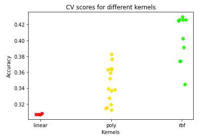
- Next, results. Different points below in a column corresponds to different hyperparameters.
- Radial basis function is the clear winner here, that allows us get to around 0.43 accuracy.
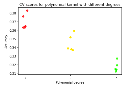
- For polynomial kernel, higher degree isn’t necessarily a good thing.
- For the gaussian used as radial bias function, the spread (controlled by gamma) does matter
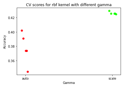
- Radial basis function is the clear winner here, that allows us get to around 0.43 accuracy.