Next we will try linear classifiers to tell the images apart. We will try a few methods here:

Multinomial logistic regression/Softmax
Support Vector Machine (SVM)
Linear Discriminant Analysis (LDA)

Of course, all of these have the assumption that our input data is “separable”. Logistic regression/SVM relies on the data being (almost) separable by a hyperplane. LDA is somewhat different; it assumes our data is generated by a few clusters, and the centers of each cluster are separated.

It doesn’t seem like people verify these assumptions in practice; a priori for arbitrary raw input, I am not convinced that this is generally the case (although empirical it seems to work fairly well). This goes back to the problem of finding good embeddings of the inputs. By composing with a “good” kernel if necessary, it is fair to say a “good” embedding should have some linear separability built in. This is perhaps why in many neural network architectures, the last layer is usually a softmax layer - one can pretend that all the previous layers try to learn a “good” embedding so that things can be linearly separated.

Remark Another desired linear property of “good” embedding is that dot product of embedding is meaningful. This is not something we need here, but it’s another major thing I don’t understand and ideally have some heuristic justification at least.

Main reference is cs231n notes

Model framework

To build a model, we will follow the framework of

finding a suitable score function to classify each input
use a suitable loss function to evaluate the model
use regularization techniques to reduce overfitting

For linear classifiers, the score function we use is an affine linear function of the inputs, hence linear.

Base case: binary logistic regression

Suppose we want to predict a binary output $y = 0$ or 1. We may model $\mathbb{P}(y = 1)$, and predict $y = 1$ whenever $\mathbb{P}(y = 1)$ is larger than some threshold. This is equivalent to model $\mathbb{P}(y = 0)$ when there are two classes, since $\mathbb{P}(y = 0) + \mathbb{P}(y = 1) = 1$.

Binary logistic regression: logit model

Suppose we want to use a linear model for this. One problem is that an affine linear function is valued in $(-\infty, \infty)$, while probability should lie in $[0,1]$. To resolve this, one can rescale $(-\infty, \infty)$ to $(0,1)$ by a nice, increasing function (so that $-\infty \to 0$, $\infty \to 1$) , i.e. take some $g: (-\infty, \infty) \to (0,1)$, and assert that

\[\mathbb{P}(y = 1) = g(a_1 x_1 + \cdots + a_kx_k)\]

if $(x_1, \cdots, x_k)$ is the input. If $g$ is invertible - then we are postulating $g^{-1} (\mathbb{P}(y = 1))$ should be linear:

\[g^{-1}(\mathbb{P}(y = 1)) = a_1x_1 + \cdots + a_kx_k\]

Common choices of $g$ are:

Expit function $g(x) = \frac{1}{1 + e^{-x}}$. Its inverse is the logit function
\[g^{-1}(p) = logit(p) = \log\left(\frac{p}{1-p}\right).\]
We can interpret this as the log odds:
\[\log \frac{\mathbb{P}(y = 1)}{\mathbb{P}(y = 0)}.\]
This is the logistic regression, and is often preferred because the logit function is the canonical link ¹ for binomial distribution. From the inference perspective, this allows us to say something like: if an input increases by 1 unit, the odds of a positive label will increase by x times.
CDF of standard Gaussian $g(x) = \frac{1}{\sqrt{2\pi}} \int_{-\infty}^x e^{-\frac{x^2}{2}} dx$. Its inverse is the probit function, and this is called the probit regression. We can think of this as a latent variable model: given input $(x_1, \cdots, x_k)$, consider the latent variable
\[y^* = a_1 x_1 + \cdots + a_kx_k + \epsilon\]
where $\epsilon \sim N(0, \sigma^2)$ is a Gaussian error, and we predict label = 1 if $y^* > 0$. This is equivalent to saying $p := probit(y^{\star}) > \frac{1}{2}$, although we should really think of this as thresholding $p$ instead, since we can move the threshold $\frac{1}{2}$ around by adding a bias/constant term in $y^*$.

The choice of probit/logistic regression is a matter of personal taste. Strictly speaking probit distribution has a slightly thinner tail, but it doesn’t matter in practice.
Log-Weibull distribution $g(x) = 1 - e^{-e^{x}}$. Its inverse is the complementary log-log function.
\[g^{-1}(p) = \log(-\log(1-p))\]
We can think of this as a latent variable model: given input $(x_1, \cdots, x_k)$, consider
\[\log \lambda = a_1 x_1 + \cdots + a_k x_k, z \sim Poisson(\lambda), y = \begin{cases} 1 & \text{ if $z > 0$} \\ 0 & \text{ if $z = 0$} \end{cases}\]
In other words, we think of the label = 1 if a certain event occurs at least once, and we model the rate of event $\lambda$ happening via $\log \lambda$ being linear over inputs.

cloglog regression is often used when the probability is either very small/very large, hence it’s pretty popular in survival analysis.²

Remark $g^{-1}$ is called the link function in generalized linear models (GLM). Stackexchange has an excellent answer on when to use which link above.

Binary logistic regression: regression - formulation of optimization problem

Recall from last section the logistic regression model: given input $\vec{x} = (x_1, \cdots, x_k)$, we model $\mathbb{P}(y = 1)$ by

\[y \vert x \sim Ber(p), \, logit(p) = a_1x_1 + \cdots a_kx_k = \vec{x}^T \vec{a}\]

for some unknown weights $\vec{a} = (a_1, \cdots, a_k)$. The next question is how to find these weights.

One common estimator is the maximal likelihood estimator - we pick the weights $\vec{a}$ so that probability of getting the empirical data is maximized. In our case, if $y \sim Ber(p)$, note that the probability of realizing an actual draw is $p$ if $y = 1$; $1 - p$ if $y = 0$. One can put this more succintly as

\[\mathbb{P}(y \vert x) = p^y(1-p)^{1 - y}\]

Now suppose we have $n$ independent data points $(\vec{x_1}, y_1), \cdots, (\vec{x_n}, y_n)$, each pair being (input, label). Due to independence, we want to maximize

\[\prod_{i=1}^n \mathbb{P}(y_i \vert x_i),\]

which is equivalent to minimizing the negative log likelihood

\[-\sum_{i=1}^n \log \mathbb{P}(y_i \vert x_i) = -\sum_{i=1}^n \left(y_i \log p_i + (1 - y_i) \log (1-p_i)\right)\]

From the information-theoretic perspective, this is the cross entropy loss. In this special case, it is exactly the KL-divergence from our predicted distribution ($p$ at label 1, $1-p$ at label 0) to the point mass of true label.

To reduce overfitting, one may want to reduce the chance for “exotic” weights to happen. What “exotic” means is subjective, but a common criterion is that weights shouldn’t be too large. Hence we may penalize weights with large norm. To do this, we may add a regularization term to the loss function:

\[-\sum_{i=1}^n \left(y_i \log p_i + (1 - y_i) \log (1-p_i)\right) + \lambda R(a_1, \cdots, a_k)\]

Our goal is then to pick weights that minimize the loss function. Note that:

The model did not change, meaning that usual ways to interpret logistic regression coefficients still apply. We merely changed the way to decide which model is the best.
Usual choice of $R(a_1, \cdots, a_k)$ are common norms on $(a_1, \cdots, a_k)$. Common in practice are $L^2$, $L^1$, elastic net and so on.³
$\lambda$ decides how strong regularization is. It is a hyperparameter that can be tuned by cross-validation.
Probabilistic interpretations of the loss function above often exists. For example, $L^2$-regularization should correspond to logistic regression, with coefficients $a_i \sim N(0, \lambda^{-2})$ (Verify?)

Binary logistic regression: regression - solving the optimization problem

Note that the loss $(a_1, \cdots, a_k) \to -\sum_{i=1}^n \left(y_i \log p_i + (1 - y_i) \log (1-p_i)\right)$ with $logit(p_i) = \vec{x_i}^T \vec{a}$ is convex. This is because

Lemma on convexity: if $f: \Omega \to \mathbb{R}$ is convex, $g: \mathbb{R} \to \mathbb{R}$ is convex non-decreasing, then $g \circ f$ is also convex.
The first part of log loss is $- \log p$, which equals
\[- \log p = - \sum a_i x_i + \log \left(1 + exp(\sum a_i x_i) \right)\]
The first part $- \sum a_i x_i$ is linear and doesn’t affect convexity. For the second part, calculus shows that $x \to \log(1 + e^x)$ is convex increasing, and so by the lemma the composition is convex. Same argument can be applied to the $- \log(1-p)$ term.

Convexity implies that to minimize the log loss, we can focus on a compact domain, hence minimum must exist. The minimum is usually not unique although, e.g. along hyperplanes where $\sum a_ix_i$ is constant. In other words, the loss is not strictly convex here.

Anyhow, even in the binary class case, exact solution doesn’t exist⁴, but we can use numerical methods to find approximate solutions. One idea is stochastic gradient descent.⁵ Same methods can be applied to regularization term as well if it exists.

Binary logistic regression: putting in the score/loss framework

Let us put the above in the score function/loss function framework we started with.

Score function: our model was
\[logit \mathbb{P}(y = 1) = \log \frac{\mathbb{P}(y=1)}{\mathbb{P}(y=0)} = a_1 x_1 + \cdots + a_k x_k\]
One way to interpret this is that⁶
- $f_i = \log \mathbb{P}(y = i)$ is the “normalized score” for class $i$.
- Logistic regression is then modeling the difference of normalized scores between class 1 and class 0.
- By a quick calculation,
\[f_1 = (a_1x_1 + \cdots + a_k x_k) - \log\left(1 + \exp(a_1x_1 + \cdots + a_kx_k)\right)\] \[f_0 = - \log\left(1 + \exp(a_1x_1 + \cdots + a_kx_k)\right)\]
- The $-\log\left(1 + \exp(a_1x_1 + \cdots + a_kx_k)\right)$ term should be thought of as a normalizing term, due to $\mathbb{P}(y = 0) + \mathbb{P}(y=1) = 1$. In this sense, we can take
\[f_1' = a_1x_1 + \cdots a_k x_k\] \[f_0' \equiv 0\]
as the “unnormalized score”. And to be honest, all we care about is the difference $f_1’ - f_0’$, and we have still done some normalization when declaring $f_0’ \equiv 0$. A cleaner way is to then treat $f_1’, f_0’$ to be both linear functions in $x_1,\cdots,x_k$, even though there is redundancy in the coefficients.
Loss function: We use the cross entropy loss as above, so one data point of $((x_1, \cdots, x_k), y)$ contributes to the loss
\[\begin{align*} - y \log p - (1-y) \log (1-p) &= - y f_1 - (1-y) f_0 \\ &= -y f_1' + \log\left(1 + \exp(a_1x_1 + \cdots + a_kx_k)\right) \\ &= -f_{y}' + \log\left(1 + \exp(f_1')\right) \end{align*}\]

Binary logistic regression: summary⁷

We formulate a logit model. This can be put in the score function framework, where the logit models difference in scores.
Finding the maximal likelihood estimator (MLE) of this model is equivalent to minimizing the cross entropy loss.
To penalize large weights, one can add a regularization term to the cross entropy loss.
To minimize the loss function, we can apply numerical methods, such as stochastic gradient descent (SGD) or Newton’s method or whatever.

Multinomial logistic regression

With the score/loss function viewpoint, the binary case generalizes readily to the multi-class case. We will sketch the relevant components here:

Multinomial logistic regression: model/score function

Suppose there are $m$ classes $0, 1, \cdots, m-1$ to classify to. Suppose also that these classes are ordinal, meaning that the order doesn’t matter. Then we can

model a classification as drawing class $i$ with probably $i$.
to model $p_i$, again take class 0 as baseline, and model
\[\frac{\log(\mathbb{P}(y = 1))}{\log(\mathbb{P}(y=0))}, \cdots, \frac{\log(\mathbb{P}(y = m-1))}{\log(\mathbb{P}(y=0))}\]
linearly in terms of input variables. More formally,
\[y|x \sim Multi(1; p_0, \cdots, p_{m-1}), \, log\left(\frac{p_j}{p_0}\right) = \vec{x_j}^T \vec{a}\]
Alternatively, we can take the score function viewpoint and model
\[\log p_i = \sum_j a_{ij} x_i + C\]
where a constant $C$ is needed to make sure $\sum p_i = 1$. Equivalently, we are modeling
\[p_i \propto e^{\sum_j a_{ij} x_i}\]

Multinomial logistic regression: formulating optimization problem

Suppose the data points are $(x_1, y_1), \cdots, (x_n, y_n)$, where $x_i$ is input, and $y_i$ are the true label (one of the classes $0, 1, \cdots, m-1$). We will use $y_{i0}, \cdots, y_{i, m-1}$ to reprsent the one-hot encoded version of $y_i$. For example, if $y_i = 1$, then $y_{i0} = y_{i2} = \cdots = y_{i,m-1} = 0$, and $y_{i1} = 1$.

Finding MLE means we want to maximize
\[\prod_{i} \mathbb{P}(y_i | x_i) = \prod_i \prod_j p_{ij}^{y_ij}\]
which is equivalent to minimizing the negative log likelihood:
\[- \sum_i \sum_j y_{ij} \log p_{ij}\]
The term $-\sum_j y_{ij} \log p_{ij}$ is the cross entropy loss of our predicted distribution $(p_{ij})$ to the point mass of true labels $(y_{ij})$.
Regularization term can be added like before.

Multinomial logistic regression: solving the optimization problem

The cross entropy loss is convex, so minimum exists, but the solution may not be unique. The exact solution doesn’t exist, but we can use numerical methods such as SGD.

For future reference, here’s the gradient of the cross entropy loss. Since my indices have been sloppy above, let’s redeclare the notations once and for all here:

$(\vec{x_1}, y_1), \cdots, (\vec{x_n}, y_n)$ are the input and true label. Each $\vec{x_i} \in \mathbb{R}^{K \times 1}$, to stress that it’s a column vector.
$\vec{y_i} = (y_{i0}, \cdots, y_{i, j-1})^T \in \mathbb{R}^{J \times 1}$ are the one-hot encoded version of $y_i$. Sometimes we use $y_i^*$ to represent the true label instead, to disambiguate from $\vec{y_i}$.
Logistic regression model is then
\[\log p_{j} \propto \sum_{k} a_{jk} x_k\]
We can form the matrix $A = (a_{jk}) \in \mathbb{R}^{J \times K}$.
Cross entropy loss is then
\[\begin{align*} - \sum_i \sum_j y_{ij} \log p_{ij} &= - \sum_i \sum_j y_{ij} \left(\sum_k a_{jk}x_{ki} - \log \left(\sum_j exp\left(\sum_k a_{jk} x_{ki}\right)\right)\right) \\ &= - \sum_i \left(\vec{y_i}^T A \vec{x_i} - y_i^* \log \sum_j \exp \left(\vec{e_j}^T A \vec{x_i}\right)\right) \end{align*}\]
Here $e_j = (0, \cdots, 1, 0)^T$ is the indicator vector in $\mathbb{R}^{J \times 1}$ with 1 at $j$-th position and 0 elsewhere.
Total derivative of the cross entropy loss is the linear map:
\[H \to - \sum_i \left(y_i^T H x_i - \frac{\sum_j e_j^T H x_i \exp(e_j^T A x_i)}{\sum_j \exp(e_j^T A x_i)}\right) = - \sum_i \left(y_i^T H x_i - \sum_j e_j^T H x_i p_{ij}\right)\]

Applying logistic regression to CIFAR-10

View notebook on binder

Let’s code! Logistic regression is implemented in most APIs, so I am not going to implement it from scratch. I will use tensorflow and explore a few questions:

Do we need to normalize the input by dividing by 255, or centering then normalize by standard deviation?
- A prior this is not clear to me, given that RGB is on a fixed scale [0,255]. Generally logistic regression needs normalization only if the scale varies for different input variables.
How do different optimizers affect things? SGD is the most naive approach, while Adam is the standard optimizer people use these days. Here is an overview of some popular optimizers by the way.⁸
How does the number of epochs affect things? This is the number of times you go through the training data.
How does regularization affect things? We will use $L^2$ here, although the comparison between $L^1$, $L^2$ and elastic net is again interesting.

Since there are many combinations of hyperparameters here, I will use tensorboard to help me figure out what is going on, following this tutorial. I look at

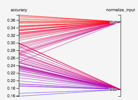
   Normalize input: yes/no
   Optimizer: Adam/SGD
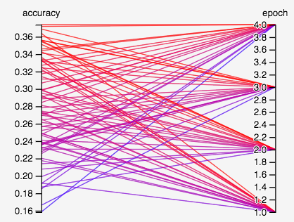
   Epoch: 1, 2, 3, 4
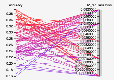
   L^2 regularization weight: 0, 0.0001, 0.001, 0.01, 0.1

To answer the questions above:

Do we need to normalize the input by dividing by 255, or centering then normalize by standard deviation?
- For gradient methods to work well, we generally want gradients to stay a bit away from zero to avoid the vanishing gradient problem. Normalizing inputs to the “activation” region of the softmax function would help this happen link. In this case, normalizing to $[0,1]$ would be sufficient.
- Empirically, looks like normalization definitely does better. The best model without normalizing input has an accuracy of ~0.3, while most models normalizing input does better than that, with the best one achieving an accuracy of 0.37.
How do different optimizers affect things?
- The biggest drawback of SGD is that learning rate is uniform for all parameters, which means picking an optimal learning rate (whatever that means) is difficult.
- Adaptive algorithms try to resolve this by keeping a per-parameter learning rate instead. This means default learning rate often works sufficiently well, so less tuning.
- However, the NIPS paper The marginal value of adaptive gradient methods in machine learning suggests that adaptive methods generalizes worse than SGD. There is also a nice blog post that supports this conclusion.
- Empirically here, SGD/Adam looks fairly similar to me.
How does the number of epochs affect things?
- It seems like as epoch increases, the variance of accuracy increases when we vary over other hyperparameters.
- There doesn’t seem to be too much gain in increasing epoch in this case. The best model with 1 epoch has accuracy ~0.364, while the best model with 4 epochs has accuracy ~0.374.
How does regularization affect things? We use $L^2$-regularization here, so let’s see if regularization helps by checking performance with no regularization (weight = 0) vs different settings of regularization weights.
- The best model without regularization has accuracy ~0.369, not far off from best model ~0.374 with regularization weight 0.0001. I didn’t look into the variance of these models, but I would assume the gain here is too small to be a conclusive gain.
- On the contrary, a regularization weight of 0.1 is likely too big. The best model with such weight has accuracy ~0.3, which is a pretty big dropoff.

Footnotes

Details ↩
No, I don’t know what I am talking about. A note here as a reminder to look this point up. ↩
Say something about empirical/theoretical behavior of regularization - e.g. lasso tends to do variable selection. What does elastic net do? ↩
Everyone claims this online, and I didn’t bother to check. ↩
Dive into basic numerical methods later. ↩
Connection of logistic regression to log-linear models - is this through the score function viewpoint, and allows more flexible modeling of $\frac{\mathbb{P}(y=1)}{\mathbb{P}(y=0)}$, or something else? Link ↩
Look at model fitting metrics (if we care about inference), e.g. goodness of fit/deviance link ↩
Look into how Adam works - or maybe adaptive optimizers in general. Also look at what SGD + Momentum means. ↩